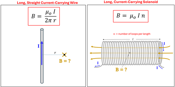
In the previous sections of this lesson, we introduced two equations that allowed us to calculate the magnetic field around wires that carry current.  The first equation allowed us to determine the magnetic field at any distance away from a long, straight current-carrying wire.  The second helped us find the magnetic field inside a long current-carrying solenoid.

When each of these equations was introduced earlier in this section, we explained that understanding where these equations come from would require us to use a relationship called Ampere’s Law.  That is the purpose of this section.  Our goal is to use Ampere’s Law to derive these two equations and show how Ampere’s Law can be applied to find the magnetic field for other current-carrying wire geometries as well.

Ampere’s Law is named after a Frech scientist named Andre-Marie Ampere.  Because of his contributions, the unit for current, the Ampere (or Amp for short), bears his name.  Ampere imagined a closed loop (sometimes called an “Amperian Loop”) of an arbitrary shape that surrounds a current.  He knew that this imaginary loop would be immersed in the magnetic field created by the current.  He next envisioned breaking the imaginary loop up into very small segments of length ∆l, where ∆l  is small enough so that the magnetic field could be considered constant over any given segment.  Ampere’s Law then states ΣB_II ∆l = μ_oI_enc. 

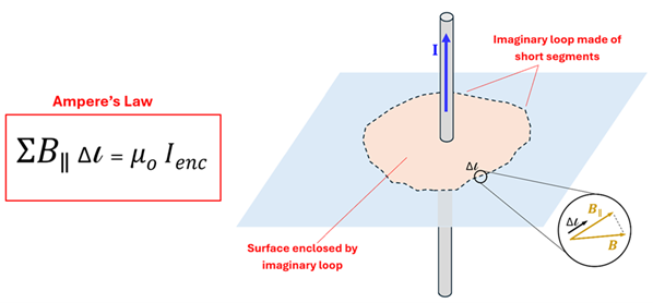
where B_II is the component of the magnetic field parallel to ∆l , I_enc is the current enclosed in the loop, and µ_o is the permeability of free space.  The summation on the left side of the equation simply means that we must add up the product of B_II and ∆l around the entire loop.  The right side of the equation consists of this familiar constant that we have seen before times the current that is enclosed by our imaginary loop.  Ampere's Law makes sense because it directly supports the idea that an electric current creates a magnetic field.  Going a step further, it states that the strength of the magnetic field is directly proportional to the current and, as we’ve already seen before, that the magnetic field circles the wire in a direction determined by the “Field-finding” Right Hand Rule.  Simply stated, the more current the stronger the magnetic field produced.  

While Ampere stated that any shaped Amperian loop can be used, applying this equation becomes much simpler if we choose the shape of our imaginary loop to satisfy one or both of these conditions:  (1) the magnetic field is a constant value and parallel to each segment around the loop, and/or (2) there is no field parallel to the loop.  To understand what these conditions mean, let’s consider two examples—the long straight wire and the solenoid.

Application of Ampere's Law

Example 1: Magnetic Field around a Long, Straight Current-carrying Wire

Problem: Use Ampere’s Law to derive an expression for the magnetic field at a distance ‘r’ from a long, straight current-carrying wire. 

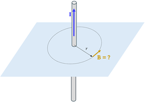
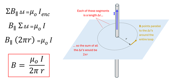
Solution:  To derive an expression for the magnetic field a distance ‘r’ from this long, straight current-carrying wire we will begin by encircling the wire with an imaginary Amperian loop.  While Ampere’s Law suggests that any imaginary closed loop will do, we will want to be very particular about the shape of the loop that we select in order to perform the summation on the left side of Ampere’s Law with relative ease.  We stated above that performing this summation is much simpler if we choose the shape of the loop such that the magnetic field is the same value at each segment ∆l  of our loop and always parallel to these segments.  A circular loop or radius ‘r’ is the shape that will satisfy this condition.  How do we know this?  We know that the magnetic field must be the same value at each segment of our imaginary loop since all these segments are the same distance ‘r’ away from the wire.  We know that the magnetic field will point parallel to each short segments, ∆l , since the magnetic field is tangent to the circle.

The good news is that if B_II is the same value at each segment, we can pull B_II out in front of the summation sign.  This is what you may have done in algebra when you added up something like (3·x) + (3·x) +(3·x) +(3·x) + ··· which would simply equal 3·(x + x + x + x + ···).  Then, all we have to do is sum up all the lengths ∆l  around our entire circular loop.  Since this is a circle, however, we know that this sum would be the circumference of a circle of radius ‘r’. Solving for B_II, which is just the magnetic field at any distance ‘r’ from the wire, gives us the same equation that we find above.

What is powerful about Ampere’s Law is that it does not just work for a long, straight wire.  It can be used to find the magnetic field around ANY configuration of current-carrying wires.  Next, let’s look at how we can apply Ampere’s Law to find the magnetic field inside a long solenoid.

Example 2: Magnetic Field Inside a Long Solenoid

Problem: Use Ampere’s Law to derive an expression for the magnetic field at a point inside a long solenoid.

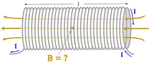
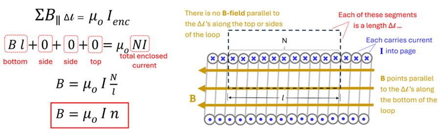
Solution: Let’s begin by imagining that we were to cut the solenoid in half by making a length-wise vertical cut down the center of the solenoid.  This cross-sectional view provides us with a very clear way to see that for each coil of this solenoid the current is pointing into the page at the top of the solenoid and out of the page at its bottom.  This is particularly helpful as we draw our imaginary Amperian loop around some of these coils that carry current.  Instead of drawing an imaginary circular loop as we did for Example 1, however, let’s draw an imaginary rectangular loop.  Why this shape?  Recall that the summation in Ampere’s Law is much simpler to apply if we choose a shape for our imaginary loop that satisfies one or both conditions mentioned above.  For this situation, we want to pick a shape so that (1) the magnetic field is a same value and always pointing parallel to each segment ∆l  along the bottom portion of our imaginary loop that is inside the solenoid.  This shape is also chosen since (2) there is no field parallel to the ∆l ’s for the top and two side segments.   

Remember that the left side of Ampere’s Law sums up the products of the magnetic field that is parallel to each of the small ∆l ’s around the loop.  As it turns out, this is not zero only for the bottom of our imaginary Amperian loop.  If we let our Amperian loop be length l, then Bl is entire sum of the bottom segments.  As we work our way up and down the side segments of our loop, we see that these segments point perpendicular (not parallel) to B.  Thus, there is no contribution to the left side of Ampere’s Law due to the two sides of the loop.  Finally, since for very long solenoids the magnetic field is essentially zero outside of the solenoid, the top portion of our imaginary loop does not contribute to our sum either.

Let’s look at the right side of Ampere’s Law next.  The right side of the equation represents the produce of μ_o times the total enclosed current, Nl. The reason we multiple the solenoid’s current by N is because each coil carries current I.  The more coils the stronger the magnetic field.

Solving the equation for B allows us to define the number of coils per length, N / l as n.  Thus, we have an expression for the magnetic field inside a solenoid—the very same equation we have shown above.

We have applied Ampere’s Law for two situations in this section.  This relation, however, can be applied to find the magnetic field around any geometry of current carrying wires.  

Check Your Understanding

Use the following questions to assess your understanding. Tap the Check Answer buttons when ready.

1. What does Ampere's Law allow us to find?

2. In Example 1, we chose a circle for the shape of our Amperian loop.  In Example 2, we chose an imaginary loop in the shape of a rectangle.  How do we decide on the best shape of the imaginary Amperian loop?

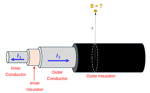
3. A coaxial cable consists of an inner conductor (a wire) that carries current in one direction that is surrounded by an outer conductor carries current in the opposite direction.  The two conductors are separated by insulating material.  Assume that the inner wire carries current I₁ to the left while the outer conductor carries current I₂ to the right.   Using Ampere’s Law, derive an expression for the magnetic field at a distance ‘r’ away from the center of this long, straight coaxial cable.

Check Answer

By drawing an end view of the wire, we can imagine an Amperian loop of radius ‘r’ circling the wire that includes the point where we want to determine the strength of the magnetic field.  The enclosed current can be thought of as the difference in the currents, I₂ - I₁ , since the inner current can be thought of ‘cancelling out’ some of the outer current as the currents are in opposite directions.  Thus, the net magnetic field, B, is just the results of the magnetic field created by the outer conductor’s current minus the magnetic field of the inner wire’s current.
A practical application of coaxial cables is to actually have both the inner and outer conductors carry the SAME current--just in opposite directions.  Can you see that the result of this is that there is no magnetic field outside of such a cable?  For sensitive electronics, this is actually important and the coaxial cable in one way to accomplish this!